PARALLEL PROGRAMMING IN R WITH PBDR PACKAGES
Introduction
R is an open source programming language and software for statistical computing. One of the biggest advantage of R is the number of libraries that it has. Similar to other interpreted programming language, R speeds tend to be slower compared to compiled programming language like Fortran, C and C++. R’s performance is also further compromised by its interpreter that only run in single thread.
Many libraries have been written to increase R’s performance, such as interface with other languages (RCpp provides interface for C++ to R) and parallel processing, such as RMpi (MPI implementation on R) and snow. The recent addition is pbdR (Programming with Big Data in R) which is spurred by the increasing trend of big data analytics. Other additions to this trend are RHadoop (R package to manage and analyze data in Hadoop) and SparkR (R package to use Apache Spark from R).
pbdR is a framework for distributed programming in R. It consists of MPI programming model, distributed matrix data structures, profilers, etc. The tools included in pbdR are listed below:
- pbdMPI (MPI interface for R)
- pbdDMAT, pbdBASE, pbdSLAP (large scale distributed matrix algebra and statistics operations)
- pbdPROF (profiling tools)
- pbdDEMO (pbdR demo)
- pbdNCDF4 (parallel I/O for NetCDF4 data)
This article will introduce pbdMPI and distributed matrix data structure.
pbdMPI
MPI implementation for pbdMPI is similar to the MPI for C, C++ and Fortran with limited abilities. The following code shows simple pbdMPI program that print the size and rank of communicators.
library(pbdMPI, quiet=TRUE)
## initialize communicator, this is needed to start pbdMPI implementation
init()

size <- comm.size() # size of communicators
rank <- comm.rank() # rank of communicators

comm.print(size)  # print only in process 0
comm.print(rank, all.rank = TRUE) # print in all other processes

finalize() # stop communicator
library(pbdMPI, quiet=TRUE)
init()

size <- comm.size()
rank <- comm.rank()

## create random number at each processors
x.local <- sample(1:size, size=1)

## reduce operation at all processors
x <- allreduce(x.local, op=’sum’)

## gather operation at all processors
x <- allgather(x.local)

## broadcast operation at all processors
if (rank == 0) {
  x.local <- 10
  bcast(x.local)
}

finalize()
pbdMPI implements MPI reduce, broadcast and gather function used to communicate data between communicators. Examples of pbdMPI reduce, broadcast and gather operations is shown below:
Other than the basic MPI functions, pbdMPI also has the implementation of “apply” function in R, (pbdApply, pbdLapply, and pbdSapply).
Distributed Matrix

pbdBASE and pbdDMAT packages provide distributed matrix data structure (ddmatrix) for R along with collections of method to perform common matrix operations, e.g. dot products, matrix factorization, etc. Data in ddmatrix are distributed along the number of processor available. The data are distributed in block distribution, cyclic distribution or block-cyclic distribution (Figure 1).
pbdBASE and pbdDMAT also provide some of the most common statistical function operated with matrix class in R, e.g. mean, max, min, etc. It also has capability in reading large data files with multiple processors and saving it to distributed matrix.
library(pbdDMAT,quiet=TRUE)
init.grid()

## create distributed random matrix
dx <- ddmatrix(rnorm(100), nrow=10,ncol=10)

## reading data with multiple processes into distributed matrix
dx <- read.csv.ddmatrix("myfile.csv ", sep = ",", nrows=10, ncols=10, header=TRUE, bldim=4, num.rdrs=2, ICTXT =0)

## statistical methods on distributed matrix
sm <- sum(dx)
mn <- mean(dx)

## matrix operation on distributed matrix
dx2 <- dx %*% dx   # dot product
dx3 <- chol(dx)    # cholesky factorization
dx4 <- dx + dx     # matrix addition

finalize()
Example: Monte Carlo Simulation
Value of π can be numerical approximated by using Monte Carlo simulation. From N number of samples of uniform observation of points inside a unit square, L number of samples that fulfill criteria are collected. Then, π can be approximated by using the following equation:
## serial monte carlo
N <- 5e8
X <- matrix(runif(N*2), ncol=2)
r <- sum(rowSums(X^2) <= 1)
PI <- 4*r/N
print(PI)


## parallel monte carlo
library(pbdMPI,quiet=TRUE)

init()

comm.set.seed(seed=1234567, diff=TRUE)

N <- 5e8
N.gbd <- N/comm.size()
X.gbd <- matrix(runif(N.gbd*2), ncol=2)
r.gbd <- sum(rowSums(X.gbd^2) <= 1)

r <- allreduce(r.gbd)

PI <- 4*r/N
comm.print(PI, quiet=TRUE)

finalize()

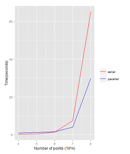
The serial and parallel R implementations for Monte Carlo simulation are shown below. The simulations are run with N’s value ofwhere. The parallel implementation is run with 4 processors. Simulations’ running time are plotted for both serial and parallel implementations (Figure 2), where it shows that the running time for both implementations are identical up to the number of points of . However, beyond the running time for serial case is significantly double the running time for parallel case.

