AI FOR HPC CLOUD RESOURCE RECOMMENDATION – AN INTERNSHIP PROJECT AT NUS IT

Introduction
The High Performance Computing (HPC) team at NUS IT provides services and resources for users to run large-scale computational jobs. These jobs range from machine learning programs to simulation programs by users from various departments. However, users may not always know the right amount of computational resources to request for their jobs, often resulting in resources requested being underutilised. With more resources requested than utilised, more unused resources are hogged on the HPC clusters than necessary which results in longer queueing times for other users waiting for their turn to run jobs.
Hence, we aim to optimise the allocation of resources to users to ensure efficient utilisation of available resources, which in turn reduces the time each user has to wait as many jobs are allowed to run as possible.
However, the problem of optimising resource allocation is a complex one. There are many factors to consider that may affect the efficiency of a computation job, and this results in a large hypothesis space for our solution to this problem, making optimisation for resource allocation rather intractable.
In order to effectively tackle such a problem, we aim to find a solution which is as optimal as possible by using modern state-of-the-art machine learning algorithms and techniques to discover insights and patterns in past data of jobs submitted that may be difficult to identify using human means. By developing a model that learns from historical data, we then use our trained model to make predictions on future jobs submitted to the HPC cluster.
Data Engineering
We first embarked on the first phase of development of our machine learning application, which is Exploratory Data Analysis (EDA) and Extraction, Transformation and Loading (ETL) of data. Through this phase, we hope to gain further insights about historical data on submitted computational tasks in order to identify the feature space that best allows our machine learning models to infer and learn from.
Firstly, the initial large feature space was reduced by extracting only the most important features. This is done by computing the correlation matrix for the original feature space and taking features that correlated highly with resource utilisation.
Since a large portion of data was skewed in terms of distribution, we also applied the appropriate data transformation to necessary features in order to normalise the spread of these features. Categorical features also had their values properly transformed and encoded.
Lastly, feature engineering was introduced in order to create new features that strengthened the correlation between the feature space and the resource utilisation. This aims to reduce the bias of the trained models during the model training phase of our development pipeline in order to produce more accurate results.
After applying these EDA and ETL techniques to the original dataset, our transformed dataset is now ready to be used for training and testing in the model development portion of the project.
Model Development
Using the insights from analysing historical data of past computational tasks submitted, we now proceed to develop an algorithm to predict the CPU efficiency as well as the computational resources that the job will utilise.
We initially began by performing exploratory modelling on various state of the art machine learning algorithms, fitting these models on our dataset that has previously undergone feature selection and data transformation. The models consist of a wide range of machine learning algorithms from Support Vector Machines to Random Forests and Gradient Boosting Machines.
The historical data is first split into a training and test set, where each model is first fit into the portion of the data for training, after which its performance is evaluated by obtaining the predictions of each model on the test data set. We use 2 metrics for evaluating the performance of each model, the first being the 𝑅2 score which explains how much the true values vary around the predictions. A higher 𝑅2 would mean less variance, and that the data is well fitted onto the model.
The second metric is the Mean-Squared Error (MSE) of the predictions. This metric measures the errors made in the prediction calculated as the difference between the prediction and the true CPU utilisation of the job. The results that we have obtained for some of the models are as follows:
| Model |
𝑅2 Score |
Mean-Squared Error (MSE) |
| Random Forest | 0.789 | 0.726 |
| Support Vector Machines (RBF Kernel) | 0.743 | 0.783 |
| XGBoost | 0.757 | 0.834 |
| CatBoost | 0.866 | 0.750 |
We can see that some of the models managed to obtain an 𝑅2 score of around 0.8, which demonstrates that these models both fit the data well, and generalises to unseen data, being the test dataset.
In the process of testing various models and their performance to generalise to unseen data, ensemble learning methods tend to perform relatively well on its own. Ensemble learning is a method whereby multiple machine learning models are put together to create a set of learners that aim to solve the same problem. In the context of aiming to optimise CPU utilisation, it is akin to having multiple experts(models) to consult regarding the prediction. Ensemble learning methods tend to cover a larger subset of the hypothesis space due to having multiple base learners that are fit on various subsets of the training data, producing a more accurate and reliable prediction that just a single base machine learning model, making it favoured as a popular machine learning algorithm for many real-world search problems today.
In order to obtain the most optimal results, we have explored various ensemble learning methods like bagging, where multiple lowly-correlated base models are trained on various subsets of the training data. The Random Forest algorithm is one example of a bagging algorithm.
Other models such as XGBoost and CatBoost are examples of models that use gradient boosting, whereby multiple learners are constructed similar to bagging. However, the difference lies therein that in boosting each consequent base learner is built upon the errors of the previous base learner, creating a sequential process of learning from past errors.
Additionally, we continue to strive to improve our prediction results by combining all the models that have performed well into a single learner by using yet another ensemble learning method: stacking.
Model stacking is an ensemble method whereby a higher level meta learner is constructed based on the predictions of the base models used.
Mathematically, if the base models are represented as functions where fi is the ith model, and represents the set of base learners, as such:

Then, for each training example 𝑥, a new feature vector ![]() is produced as follows by obtaining the prediction of each base model fi on the training example 𝑥:
is produced as follows by obtaining the prediction of each base model fi on the training example 𝑥:

This new feature vector ![]() is used as a training example for the second-level L2 meta learner which produces a prediction value ypred based on
is used as a training example for the second-level L2 meta learner which produces a prediction value ypred based on ![]() as input features.
as input features.

Where the L2 meta learner can be represented as a vector of weights ![]() .
.
An overview of the prediction pipeline that we used in stacking the base models can be viewed as follows:

With model stacking, the L2 model is able to identify different possible subspaces that each base model encompasses from the entire hypothesis space, and which model performs well in which subspace. For example, if the ith model is able to make accurate predictions for subspaces of the hypothesis space involving the feature xj , then the L2 model is able to learn and take advantage of that.
For our second-level model, we have decided to use XGBoost to learn from the predictions from our base learners, which upon training on said predictions produced the following results:
| Score | Mean-Squared Error (MSE) |
| 0.855 | 0.529 |
Here, we a drastic improvement in both the 𝑅2 score and MSE of the stacked XGBoost model over the original base models that this second-level model has learnt from.
This allows us to combine the information learned from each base model effectively with minimal loss. Using the APIs from Scikit-Learn, XGBoost and CatBoost, we have developed a stacked machine learning model in our application that outperforms the base models implemented using these machine learning libraries.
Hyperparameter Tuning
After tuning the parameters of the models through the training phase, it seems like we now have a solution to our problem. However, in our search for a solution to model our data, we encounter yet another search problem: Finding the best hyperparameters.
Hyperparameters, unlike the usual parameters that correspond the weights for each of the features, are properties that cannot be learned by the model during the training phase. These parameters may control other aspects of the model, such as how complex the overall model is or how quickly it converges to a local minimum. Since they cannot be learned by the model, we must manually tweak these settings in order to obtain the best overall results for our models.
Traditionally, grid search and/or random search has been widely used to tune hyperparameters of various models by providing combinations of hyperparameters to try, and then picking the best combination that yields the best results for that model. However, handpicking grids of hyperparameters from a huge available space may not always yield the best results even for the most experienced of data scientists and engineers. Given the large space of hyperparameters for a single model, it would be time and resource consuming to do a grid search over combinations of hyperparameters that might not necessarily provide an optimal solution. Therefore, we have decided to opt for a smarter search over the available hyperparameter space using Bayesian Optimization.
Bayesian Optimisation is a technique that does a search over the solution space based on prior beliefs about the solution space inferred from data and produces an updated posterior belief that tells us which solution is most optimal after observing past data. This is achieved using a trade-off between exploring the available hyperparameter space and exploiting what is expected to maximise our results. Among the variants of Bayesian Optimization, we have chosen an algorithm using Gaussian Processes to model the solution space for our hyperparameters, using an acquisition function of Expected Improvement. This was implemented in our application using the Scikit-Optimise API. Through Bayesian Optimization using Gaussian Processes, we were able to search over a greater hyperparameter space that is not limited to a grid provided and obtain a probabilistically optimal set of hyperparameters for each model that performs at least as fast as random search. This both justifies the optimality of results from hyperparameter tuning and consumes less time.
Deployment
After training and tuning both the base learners and second level meta learner, we now have the components ready to develop our application for deployment. The resource recommendation tool is developed in Python, which utilises the prediction of the computational resources of a submitted job script produced by our machine learning model as the core feature.
Aside from the prediction made by our model, the resource recommendation tool also optimises the resource utilisation of a submitted job script before and after the recommendation using the predicted resources in various areas such as accounting for the HPC cluster, queue and node used, as well as providing custom metrics to evaluate resource utilisation. For example, we measure the efficiency of CPU utilisation of a specific job script as such:

Where 𝐸ffi represents the CPU utilisation efficiency of the ith job script submitted, penalised as the job submitted wastes more resources than needed, and if the job script hogs too many nodes in a cluster.
The deployment phase was another bottleneck in the development pipeline aside from training our models, as there were multiple additional factors to consider which now included usability and intractability of our resource recommendation tool.
The first of our concerns was the fact that there were multiple environments and versions of Linux and Python across the HPC clusters and nodes available for use. This could affect the availability of our resource recommendation tool for use to the public using specific clusters where the necessary dependencies are not pre-installed on the cluster, or if the environment is not compatible with our tool. Using different environments could also result is slightly different experiences across the clusters if the tool is deployed separately on each cluster.
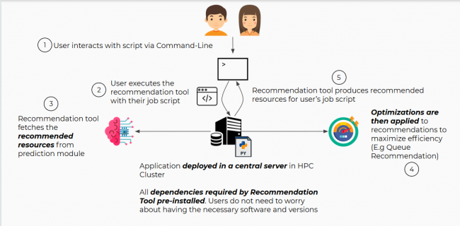
To combat this scenario, we have deployed our tool in a central location, which has all the dependencies needed to produce the resource recommendation. Users will then obtain the recommended resources for their computational job by executing the tool from any cluster that they are on without worrying about having the necessary dependencies installed on the cluster they use.
As an application that aims to improve user experience on HPC clusters, the user interaction with the resource recommendation tool is another area of concern during the development and deployment of this application. During deployment and testing, we strive to improve the speed and performance of the tool to the best of our ability by making tweaks and optimisations to decrease the wait time the user has to wait when running the resource recommendation tool, as well as providing various options for the user apart from resource recommendation for their job script. This is showcased by the option to generate the recommendation for which cluster or queue to use for their job.
To use the resource recommendation tool on the HPC cluster, enter the following command:
rectool <job_script>.pbs
Where <job_script> is the job script for which the recommendation will be generated for. Upon executing the recommendation tool via this command, the tool will generate the recommended resources for the provided job script.

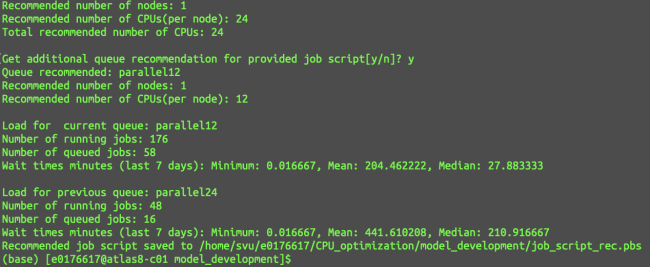
Depending on the queue that is specified in the job script, the resource recommendation tool will also prompt the user if an additional recommendation for which queue to be used for submitting the job to should be generated as well. In this example, we shall accept the recommendation for the queue in addition to the resources, which produces the following output:

The resource recommendation tool then generates a job script with the recommended resources, and queue if the queue recommendation is accepted and saves it to the same directory as the original job script.
In addition, statistics for the queues are also provided to let the user see the changes in the waiting time for the queue that is used. From the image above, we can see that accepting the recommendation for the queue puts the computational task on a queue with lesser wait time on average. The user is then less likely to wait longer for their jobs to run and subsequently complete.
Conclusion
During the development of the resource recommendation tool, we have obtained many interesting insights and from exploring historical data of jobs submitted to HPC, as well as from testing and tuning machine learning models using this data. The discoveries made during this project allowed us at HPC to better understand the nature of the problem of improving resource utilisation and allocation on HPC clusters, which in turn equips us to effectively tackle this optimisation problem, achieving a high 𝑅2 score of around 0.85 on our final machine learning model.
Moving forward, we aim to take the insights and heuristics attained from this project with us and continue to seek further improvement by not only continuing to improve our resource recommendation tool, but also apply transfer learning by exploring new areas for which we can apply our newfound understanding of such optimisation problems to problems of other domains of a similar nature.
Should there be any further enquiries, do feel free to contact the HPC Data Engineering team at DataEngineering@nus.edu.sg.

